Least Square Method
The least squares method is a fundamental approach in data fitting. Although it is quite simple, the way different people observe and learn about the same algorithm can vary significantly. Therefore, I believe it is necessary to organize my understanding of the least squares method here.
The simplest problem in data fitting is linear fitting. For example, consider the following sampled data:
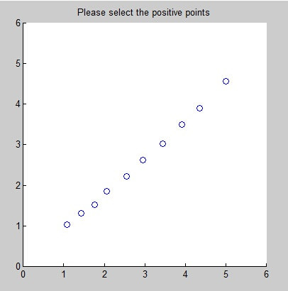
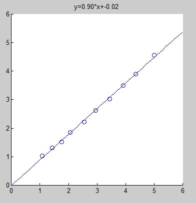
We hope to achieve the following effect through linear fitting:
We define these data points as $(x_1,y_1),(x_2,y_2),…,(x_N,y_N)$, and let the fitted line be
$$ f(x)=a \times x+b $$
We definitely want the discrete points to be as close to the line as possible. In mathematical terms, this can be expressed as:
$$ \min E(a,b) $$
where
$$ E(a,b) = \sum_{n=1}^{N}(y_n-(a\cdot x_n+b))^2 $$
Matrix Form Solution
This is the essence of the least squares method. Next, we need to use this expression to solve for parameters $a$ and $b$. Personally, I prefer the conciseness of matrices, so I will express the above equation in matrix form.
$$ E(a,b) = \lVert { \begin{pmatrix} y_1 \\ y_2 \\ \vdots \\ y_N \end{pmatrix} - \begin{pmatrix} x_1 & 1 \\ x_2 & 1 \\ \vdots & \vdots \\ x_N & 1 \end{pmatrix} \begin{pmatrix} a \\ b \end{pmatrix} } \rVert_2^2 $$
We denote the vector concerning $y$ as $\mathbf{y}$; the matrix concerning $x$ as $\mathbf{X}$; and the parameter vector as $\mathbf{\alpha}$. Thus, the least squares problem is transformed to:
$$ \min_{\mathbf{\alpha}} {\lVert \mathbf{y} - \mathbf{X}\mathbf{\alpha}\rVert}_2^2 $$
Here, $\mathbf{y}$ and $\mathbf{X}$ are known quantities, while $\mathbf{\alpha}$ is the unknown. This representation is somewhat unconventional, so I will make a substitution: replace $\mathbf{X}$ with $\mathbf{A}$ and $\mathbf{\alpha}$ with $\mathbf{x}$. The problem now looks cleaner:
$$ \min_{\mathbf{x}} {\lVert \mathbf{y} - \mathbf{A}\mathbf{x}\rVert}_2^2 $$
Next, we need to solve this equation. The method is straightforward: take the derivative and set it to zero:
$$ -2\mathbf{A^Ty}-2\mathbf{A^TAx}=0 $$
Thus,
$$ \mathbf{x} = (\mathbf{A^TA})^{-1}\mathbf{A^Ty} $$
So, can the least squares method only be used for linear fitting? Not at all. It can also be used for any fitting where the parameters are linear. For example, in polynomial fitting:
$$ f(x) = a_nx^n+a_{n-1}x^{n-1} +\cdots+a_1x^1+a_0 $$
Always remember that we are solving for the parameters $a_0, a_1, \cdots , a_n$, not $x$. In this equation, the highest degree of the parameter is 1, so it can indeed be solved using the least squares method.
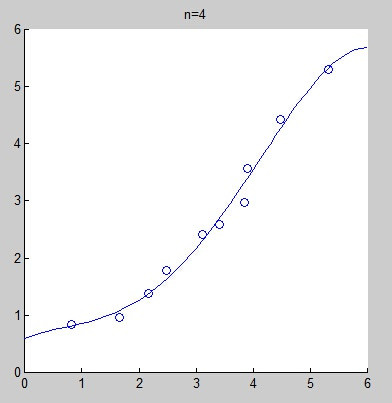
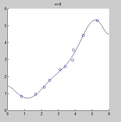
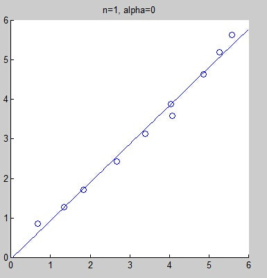
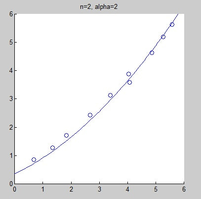
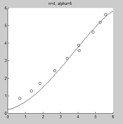
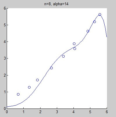
However, selecting an incorrect fitting model may lead to underfitting or overfitting. The following graphs show fitting curves obtained from the same data set using linear fitting, quadratic fitting, fourth-degree fitting, and eighth-degree fitting. Intuitively, it is hard to judge whether linear fitting is underfitting, but we can confidently say that the eighth-degree fitting is overfitting.
Of course, we can address the so-called overfitting problem by adding a regularization term:
$$ \min_{\mathbf{x}} {\lVert \mathbf{y} - \mathbf{A}\mathbf{x}\rVert}_2^2 + {\alpha \lVert \mathbf{x} \rVert}_2^2 $$
The principle behind this is straightforward and is explained in detail in both machine learning textbooks and engineering optimization texts, so I won’t elaborate on it here. Taking the derivative of the above expression with respect to $\mathbf{x}$, we have:
$$ -2\mathbf{A^Ty}+2\mathbf{A^TAx}+2\alpha\mathbf{Ix} $$
Setting the above expression to zero gives us:
$$ \mathbf{x} = (\mathbf{A^TA}+\alpha\mathbf{I})^{-1}\mathbf{A^Ty} $$
As we can see, the results have improved, but this approach may not solve all problems.
Non-Matrix Solution
The matrix solution is quite elegant, reducing the problem to a simple equation. For programming with matrices in C++, two libraries are commonly recommended. One is OpenCV’s Mat class, which can be used directly if you are already working with an image processing library. The other is Eigen, which is smaller and specifically designed for matrix calculations. However, in DSP programming, we may not need such sophistication; we just need speed.
To recap, we are solving the linear fitting problem, which can be expressed as $y=kx+b$. The target function corresponding to the least squares method is:
$$ f(k,b) = \sum_i{(y_i-kx_i-b)^2} $$
We want to know when $f$ can achieve its minimum value, so we take the derivative:
$$ \frac{\partial{f(k,b)}}{\partial{k}}=-2\sum_i{(y_i-kx_i-b)x_i} $$
$$ \frac{\partial{f(k,b)}}{\partial{b}}=-2\sum_i{(y_i-kx_i-b)} $$
Next, we set the derivatives to zero to find the extremum:
$$ \sum_i{(y_i-kx_i-b)x_i} = 0 $$
$$ \sum_i{(y_i-kx_i-b)} = 0 $$
Finally, we obtain the results:
$$ k=\frac{n\sum_i^n{x_iy_i}-\sum_i^n{x_i}\sum_i^n{y_i}}{n\sum_i^n{x_i^2-(\sum_i^n{x_i})^2}} $$
$$ b=\frac{\sum_i^n{y_i}}{n}-k\frac{\sum_i^n{x_i}}{n} $$
Weighted Least Squares
The target function in this case is:
$$ f(k,b) = \sum_i{w_i(y_i-kx_i-b)^2} $$
We proceed by taking derivatives:
$$ \begin{align} \frac{\partial{f(k,b)}}{\partial{k}}&=-2\sum_i{w_i(y_i-kx_i-b)x_i} \\ \frac{\partial{f(k,b)}}{\partial{b}}&=-2\sum_i{w_i(y_i-kx_i-b)} \end{align} $$
We set the derivatives to zero and solve for $k$ and $b$:
$$ k=\frac{\sum_i{w_i}\sum_i{w_ix_iy_i}-\sum_i{w_ix_i}\sum_i{w_iy_i}}{\sum_i{w_i}\sum_i{w_ix_i^2}+\sum_i{w_i^2x_i^2}} $$
$$ b=\frac{\sum_i{w_iy_i}-k\sum{w_ix_i}}{\sum_i{w_i}} $$
In matrix form, this can be represented as:
$$ \min_{\mathbf{x}} (\mathbf{y} - \mathbf{A}\mathbf{x})^T\mathbf{W}(\mathbf{Ax}-\mathbf{y}) $$ where
$\mathbf{W}$ is a diagonal matrix.
The final solution is:
$$ \mathbf{x}=(\mathbf{A}^T\mathbf{WA})^{-1}\mathbf{AWy} $$